Scientific Machine Learning
In my spare time I am independently conducting research on NCDEs and UDEs. 🌀
The most up-to-date list of my publications can be found on ADS or arXiv. I have not published since my PhD (2018-2023). I will update this page when I push something new out!
List of SciML related publications (+ denotes co-authors):
- Nguyen, ICML 2023 Workshop on Machine Learning for Astrophysics
- Nguyen+, NeurIPS 2023 Workshop on Machine Learning and the Physical Sciences
🎧🪴💻☕️🎧🪴💻☕️🎧🪴💻☕️🎧🪴💻☕️🎧🪴💻☕️🎧🪴💻☕️🎧🪴💻☕️🎧🪴💻☕️
Example
I provide an example of a Controlled Neural ODE learning the classic, textbook-favorite, physical system: a harmonic oscillator.
Brief introduction of Neural ODEs
Given a state $y$, the rate of change of state $y$ is described by a differential equation as $$ \frac{dy}{dt} = f(y,t) $$ The solution is obtained by forward time integration as $$ y_{t} = y_0 + \int_{t_0}^{t_f} dt \ f(y,t) $$ From an ODE perspective, a Neural ODE simply replaces analytic function(s) $f(y,t)$ with a universal function approximator - a Neural Network ($\mathrm{NN}$), which will also be a function of $y$ and $t$ as $$ \frac{dy}{dt} = \mathrm{NN}(y,t) \quad \quad \quad y_t = y_0 + \int_{t_0}^{t_f} dt \ \mathrm{NN}(y,t) $$ The usage of $\mathrm{NN}(y,t)$ can be advantageous over known physics $f(y,t)$ if the existing physics does not adequately describe reality, or if the existing known physics is too computationally expensive to use (e.g., interactions involving integrals).
A controlled ODE expands upon the definition of an ODE by allowing the RHS of the differential equation to take input controls $u(t)$ as
$$ \frac{dy}{dt} = f(y,u,t) \quad \quad \mathrm{with \ solution} \quad \quad y_{t} = y_0 + \int_{t_0}^{t_f} dt \ f(y,u,t). $$
Similar to ODEs and NODEs, the neural network in a CNODE replaces the RHS of the differential equation as $$ \frac{dy}{dt} = \mathrm{NN}(y,u,t) \quad \quad \mathrm{with \ solution} \quad \quad y_t = y_0 + \int_{t_0}^{t_f} dt \ \mathrm{NN}(y,u,t) $$
In this example, the neural ODE models here evolve a state and are trained against a truth state (i.e., is a regression problem where the hidden state is the physical state). It is important to note that neural ODE models can also be extended to other ML problems such as classification, density estimation, etc. From an ML perspective, Neural ODEs are the continuous analog of a Residual Neural Network (ResNet) and can be trained using constant memory using the adjoint method.
Note the CNODE presented above is not to be confused with a Neural Controlled Differential Equations (NCDE). From an ML perspective, a NCDE is the continuous analog of a Recurrent Neural Network (RNN) and can also be trained using the adjoint method.
Example of a CNODE to learning a 1D Damped and Forced Harmonic Oscillator
The acceleration of a mass of mass $m$, with spring constant $k$, damping coefficient $c$, and forcing force $u$ is given by $$ F_\mathrm{net} = m a \quad \rightarrow \quad \frac{d^2x}{dt^2} = \frac{-k \ x - c v + u}{m} $$ Maintaining the convention in the introduction above, the state vector $y$ contains both positions $x$ and velocity $v$ and the forcing function $u$ are the input controls. We then do the standard procedure of reducing the second order differential equation into two first order differential equations as $$ \frac{dx}{dt} = v \quad \quad \mathrm{and} \quad \quad \frac{dv}{dt} = \frac{-k \ x - c v + u}{m} $$
This physical system can be written in PyTorch as
class MassSpringDamperDynamics(nn.Module):
    def __init__(self, mass=1.0, spring_k=2.0, damping_c=0.5):
        super().__init__()
        self.m = mass
        self.k = spring_k
        self.c = damping_c

    def forward(self, t, y, u):
        x = y[..., 0:1]
        v = y[..., 1:2]
        dx_dt = v
        dv_dt = (-self.k * x - self.c * v + u) / self.m
        return torch.cat([dx_dt, dv_dt], dim=-1)
Below is an aniamtion of one mass with certain initial conditions ($x_0$, $y_0$) and physical parameters ($m, \ k, \ c$) undergoing its $t_f=5$ second trajectory.

The arrow represents the forced input $u(t)$ and the x-axis is the displacement from equillibrium.
With additional code, we can use this defined physical system to generate a batch of trajectories with different initial conditions ($x_0, y_0$) and different physics parameters ($m, \ k, \ c$).
This will be the “truth” data from which our neural model attempts to learn dynamics from. We will train on the entire batch of trajectories, leveraging’s PyTorch’s torchdiffeq package to easily integrate a batch of initial conditions forward in time.
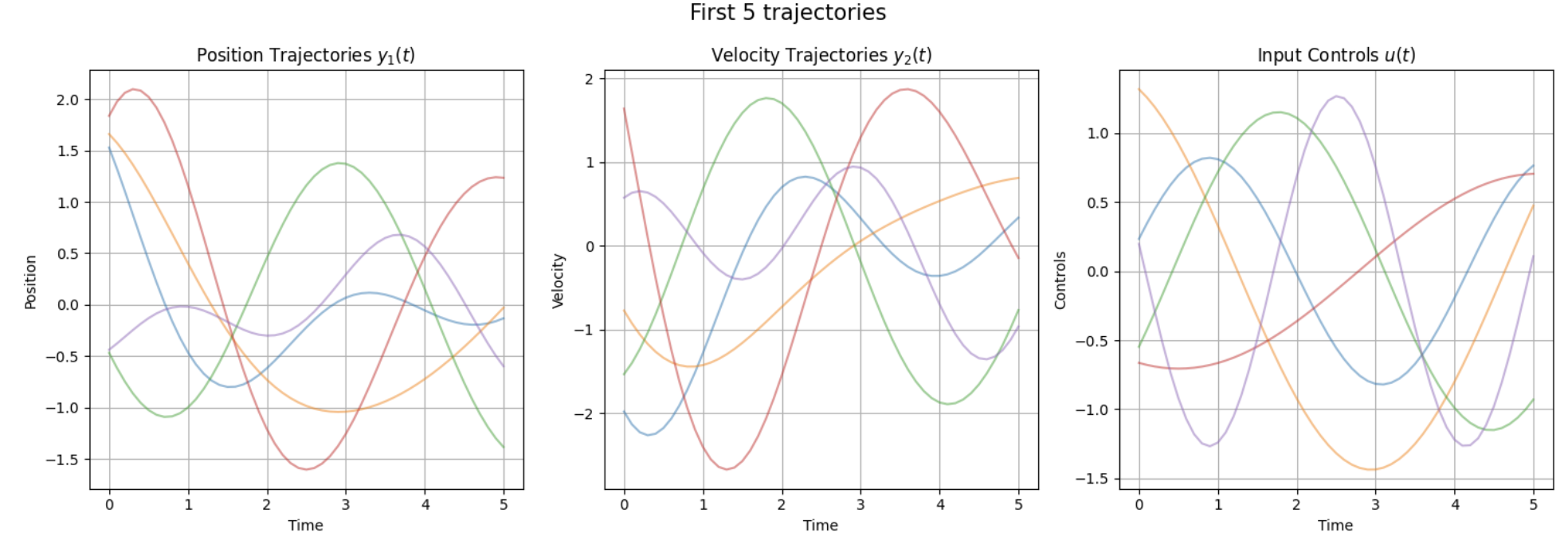
Note the first index of a tensor in PyTorch describes the batch dimension. Our truth data is then of shape y_truth.shape = [batch size, number of timesteps, state dim]. In this exmaple, I generate 50 trajectories, each with randomized initial conditions and randomized control inputs to train on. Below are the first 5 trajectories.


Now to define the Controlled Neural ODE.
class ControlledNeuralODEFunc(nn.Module):
    def __init__(self, hidden_dim=16):
        super().__init__()
        self.acc_net = nn.Sequential(
            nn.Linear(3, hidden_dim),
            nn.Tanh(),
            nn.Linear(hidden_dim, hidden_dim),
            nn.Tanh(),
            nn.Linear(hidden_dim, 1)
        )
        last_layer = self.acc_net[-1]
        nn.init.uniform_(last_layer.weight,-1e-7,1e-7)
        self.control = None
        self.dt = None

    def forward(self, t, y):
        x = y[..., 0:1]
        v = y[..., 1:2]
        u = interpolate_control(t, self.control, self.dt).unsqueeze(-1)

        xu = torch.cat([x, v, u], dim=-1)  # [batch_size, 3]

        dx_dt = v
        dv_dt = self.acc_net(xu)

        return torch.cat([dx_dt, dv_dt], dim=-1)

class ControlledNeuralODE(nn.Module):
    def __init__(self, func):
        super().__init__()
        self.func = func

    def forward(self, t_span, y0, control):
        self.func.control = control
        self.func.dt = 0.1
        pred = odeint(self.func, y0, t_span, method='rk4', options={'step_size': self.func.dt})
        return pred.transpose(0, 1)
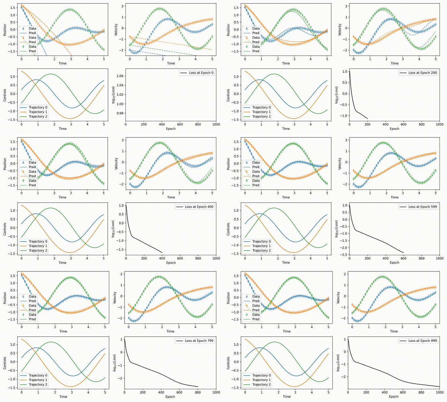
All that is left is to train the model. I use 2000 epochs for this demonstration of fitting the training data. Below is a gif of the training for the 3 trajectories above, for the first 1000 epochs. Again, during training all initial conditions are simulationeously evolved forward per timestep using their respective controls. The loss is evaluated over all trajectories over both position and velocity states over all time.

It is apparent that the neural network $\mathrm{NN}(y,u,t)$, when given controls $u(t)$, appears to have learned the dynamics of the model enough to fit the training data. A more careful treatment is required to evaluate performance outside of the training data, but is well-beyond the scope of this example.
Here is a static comparison between trained and untrained neural ODEs.

PhD Research (2018-2023)
During my time at Ohio State University, I worked with Professor Todd Thompson in computational astrophysics and used multi-dimensional simulations to better understand how galaxies launch out multi-phase galactic winds, which is ultimately connected to understanding how galaxies evolve. In the last two years of my PhD, I pivoted over to SciML research with emphasis on Neural ODEs and Universal Differential Equations.
Universal Differential Equations are a more general form of the Neural ODE discussed above, where rather than parameterize the entire RHS of an ODE with a neural network, we chose to parametrize only portions of the RHS of the ODE with a neural network(s). That is:
$$ \frac{dy}{dt} = f(y,t)_{\mathrm{existing \ physics}} + \mathrm{NN}(y,t) $$
This method leverages existing domain knowledge and incorporates a more interpretable method of including data-driven modeling. Many works often use UDEs for discovery, where Symbolic Regression (SR) is applied on the trained neural component to extract interpretable, and easily trasnferrable, analytical functions of the learned physics.
I applied Universal Differential Equations (UDEs) to study galactic outflow physics using X-ray data. UDEs embed neural networks within differential equations, allowing us to learn unknown physical terms from observational data. While traditional approaches require developing new analytical models to explain X-ray measurements of temperature and density along galactic outflow paths, UDEs combine domain knowledge with data-driven modeling. I demonstrate that this hybrid approach effectively discovers underlying physics even from a single trajectory of observational data.
3D Time Dependent Galactic Wind Simulations and Semi-Analytic 1D Models
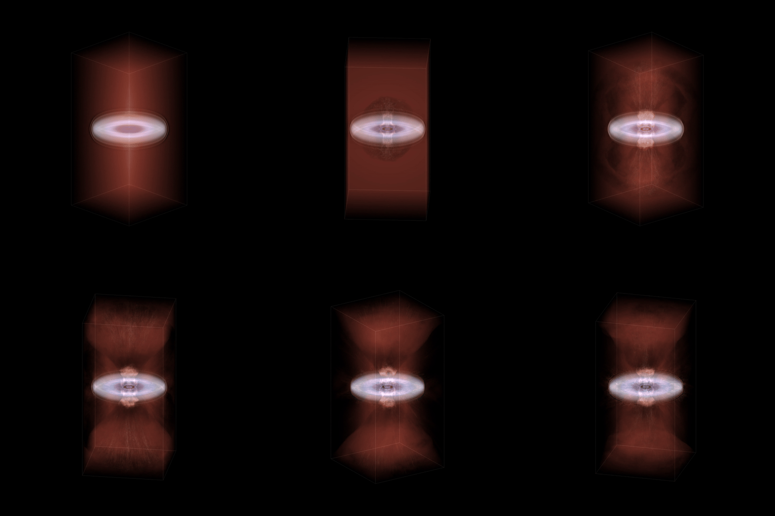
Most of my other papers are focused either on using the Cholla astrophysical code to simulate galactic winds, or using simple 1D steady state models (like the one used in the NeurIPS and ICML papers) to draw qualitative conclusions on physics related to hot galactic winds. Below is an example of a 3D render of one of my galactic wind simulations using the yt python package.
